CSV ファイルのヘッダ行をカラム名に使う

この記事は Apache Drill Advent Calendar 2015 の2日目の記事です。

11月の Tokyo Apache Drill Meetup で出た質問の中に、「CSV ファイルのヘッダ行をカラム名に使いたいが可能か?」というものがありましたが、Drill 1.2 では先頭行をスキップするオプションはあったものの、行の内容をカラム名として使う機能は未実装でした。で、その後リリースされた Drill 1.3 の [DRILL-951] CSV header row should be parsed にて、その機能が追加されたので紹介します。

例えばこんなデータがあるとします。

$ head /tmp/personal_information.csv
連番,氏名,氏名(カタカナ),性別,電話番号,郵便番号,住所1,住所2,住所3,住所4,住所5,生年月日
1,佐川邦男,サガワクニオ,男,0959408329,852-8007,長崎県,長崎市,江の浦町,2-18,江の浦町スカイ401,1995/03/28
2,松本冨子,マツモトトミコ,女,0957833608,855-0882,長崎県,島原市,札の元町,3-13,,1978/10/06
3,内田史織,ウチダシオリ,女,0942977483,848-0133,佐賀県,伊万里市,黒川町真手野,3-5-1,,1989/05/25
4,曽根里沙,ソネリサ,女,0271234470,378-0077,群馬県,沼田市,石墨町,1-7-1,パーク石墨町204,1985/03/22
5,徳田雪乃,トクダユキノ,女,083932164,752-0980,山口県,下関市,長府黒門町,3-6-5,,1988/03/23
6,山下直人,ヤマシタナオト,男,099655084,891-1206,鹿児島県,鹿児島市,皆与志町,2-10-9,ザ皆与志町314,1956/05/11
7,真田敬三,サナダケイゾウ,男,0766626361,936-0827,富山県,滑川市,東福寺,2-8-14,タウン東福寺202,1972/12/10
8,山形順子,ヤマガタジュンコ,女,0194190969,020-0851,岩手県,盛岡市,向中野,4-1-20,向中野マンション407,1979/11/21
9,奥照雄,オクテルオ,男,0895179833,799-1361,愛媛県,西条市,広江,2-5-17,広江シティ215,1987/03/17

単純に Drill で SELECT * するとこんな風になります。

0: jdbc:drill:zk=local> SELECT * FROM dfs.`/tmp/personal_information.csv` LIMIT 10;
+--------------------------------------------------------------------------------------------------------------+
|                                                   columns                                                    |
+--------------------------------------------------------------------------------------------------------------+
| ["連番","氏名","氏名(カタカナ)","性別","電話番号","郵便番号","住所1","住所2","住所3","住所4","住所5","生年月日"]                             |
| ["1","佐川邦男","サガワクニオ","男","0959408329","852-8007","長崎県","長崎市","江の浦町","2-18","江の浦町スカイ401","1995/03/28"]      |
| ["2","松本冨子","マツモトトミコ","女","0957833608","855-0882","長崎県","島原市","札の元町","3-13","","1978/10/06"]               |
| ["3","内田史織","ウチダシオリ","女","0942977483","848-0133","佐賀県","伊万里市","黒川町真手野","3-5-1","","1989/05/25"]            |
| ["4","曽根里沙","ソネリサ","女","0271234470","378-0077","群馬県","沼田市","石墨町","1-7-1","パーク石墨町204","1985/03/22"]         |
| ["5","徳田雪乃","トクダユキノ","女","083932164","752-0980","山口県","下関市","長府黒門町","3-6-5","","1988/03/23"]               |
| ["6","山下直人","ヤマシタナオト","男","099655084","891-1206","鹿児島県","鹿児島市","皆与志町","2-10-9","ザ皆与志町314","1956/05/11"]    |
| ["7","真田敬三","サナダケイゾウ","男","0766626361","936-0827","富山県","滑川市","東福寺","2-8-14","タウン東福寺202","1972/12/10"]     |
| ["8","山形順子","ヤマガタジュンコ","女","0194190969","020-0851","岩手県","盛岡市","向中野","4-1-20","向中野マンション407","1979/11/21"]  |
| ["9","奥照雄","オクテルオ","男","0895179833","799-1361","愛媛県","西条市","広江","2-5-17","広江シティ215","1987/03/17"]          |
+--------------------------------------------------------------------------------------------------------------+
10 rows selected (0.34 seconds)

各行は配列型になっているので、各カラムにアクセスするには添字が必要でした。

0: jdbc:drill:zk=local> SELECT columns[1] AS 氏名, columns[4] AS 電話番号
. . . . . . . . . . . > FROM dfs.`/tmp/personal_information.csv`
. . . . . . . . . . . > WHERE columns[1] LIKE _UTF16'田中%';
+-------+-------------+
|  氏名   |    電話番号     |
+-------+-------------+
| 田中優| 011944797   |
| 田中伍朗  | 0864019970  |
| 田中啓司  | 097833684   |
+-------+-------------+
3 rows selected (0.223 seconds)

が、バージョン1.3以降では、ファイルの拡張子をcsvhにしておくと・・・

$ mv /tmp/personal_information.csv /tmp/personal_information.csvh

これだけで先頭行がカラム名としてセットされ、クエリの中で利用できるようになります。こいつは便利ですね!

0: jdbc:drill:zk=local> SELECT * FROM dfs.`/tmp/personal_information.csvh` LIMIT 10;
+-----+-------+-----------+-----+-------------+-----------+-------+-------+---------+---------+--------------+-------------+
| 連番  |  氏名   | 氏名(カタカナ)  | 性別  |    電話番号     |   郵便番号    |  住所1  |  住所2  |   住所3   |   住所4   |     住所5      |    生年月日     |
+-----+-------+-----------+-----+-------------+-----------+-------+-------+---------+---------+--------------+-------------+
| 1   | 佐川邦男  | サガワクニオ    || 0959408329  | 852-8007  | 長崎県   | 長崎市   | 江の浦町    | 2-18    | 江の浦町スカイ401   | 1995/03/28  |
| 2   | 松本冨子  | マツモトトミコ   || 0957833608  | 855-0882  | 長崎県   | 島原市   | 札の元町    | 3-13    |              | 1978/10/06  |
| 3   | 内田史織  | ウチダシオリ    || 0942977483  | 848-0133  | 佐賀県   | 伊万里市  | 黒川町真手野  | 3-5-1   |              | 1989/05/25  |
| 4   | 曽根里沙  | ソネリサ      || 0271234470  | 378-0077  | 群馬県   | 沼田市   | 石墨町     | 1-7-1   | パーク石墨町204    | 1985/03/22  |
| 5   | 徳田雪乃  | トクダユキノ    || 083932164   | 752-0980  | 山口県   | 下関市   | 長府黒門町   | 3-6-5   |              | 1988/03/23  |
| 6   | 山下直人  | ヤマシタナオト   || 099655084   | 891-1206  | 鹿児島県  | 鹿児島市  | 皆与志町    | 2-10-9  | ザ皆与志町314     | 1956/05/11  |
| 7   | 真田敬三  | サナダケイゾウ   || 0766626361  | 936-0827  | 富山県   | 滑川市   | 東福寺     | 2-8-14  | タウン東福寺202    | 1972/12/10  |
| 8   | 山形順子  | ヤマガタジュンコ  || 0194190969  | 020-0851  | 岩手県   | 盛岡市   | 向中野     | 4-1-20  | 向中野マンション407  | 1979/11/21  |
| 9   | 奥照雄   | オクテルオ     || 0895179833  | 799-1361  | 愛媛県   | 西条市   | 広江      | 2-5-17  | 広江シティ215     | 1987/03/17  |
| 10  | 三木安弘  | ミキヤスヒロ    || 0968649092  | 865-0008  | 熊本県   | 玉名市   | 石貫      | 2-20    | 石貫ハウス107     | 1966/06/17  |
+-----+-------+-----------+-----+-------------+-----------+-------+-------+---------+---------+--------------+-------------+
10 rows selected (0.666 seconds)

ちょっとだけ説明を付け加えると、この機能はストレージプラグインのフォーマット設定にある extractHeader というプロパティで有効になります。Embedded モードで起動している場合には、Drill シェル動作中にブラウザで http://localhost:8047 にアクセスし、「Storage」タブの「dfs」プラグインの設定を見てみると、csvh の拡張子がついている場合には機能が有効になることがわかります。

  "formats": {
    ...
    "csvh": {
      "type": "text",
      "extensions": [
        "csvh"
      ],
      "extractHeader": true,
      "delimiter": ","
    }
  }

Apache Drill 今日の一言 (MOTD)

この記事は Apache Drill Advent Calendar 2015 の1日目の記事です。

Drill のフロントエンド(シェル)である sqlline を起動すると、プロンプトの前に短いメッセージが表示されます。

$ sqlline -u jdbc:drill:zk=local
Dec 1, 2015 2:13:59 AM org.glassfish.jersey.server.ApplicationHandler initialize
INFO: Initiating Jersey application, version Jersey: 2.8 2014-04-29 01:25:26...
apache drill 1.3.0 
"this isn't your grandfather's sql"
0: jdbc:drill:zk=local>

これはいわゆる MOTD (Message of the Day) と呼ばれるもので、起動のたびにランダムに選ばれたメッセージが出てきます。

「これはお前のおじいちゃんの時代の SQL ではない!」

あれ、SQL ってそんな古い時代からあったっけ?(笑)

さて、何度も起動してみると色々なメッセージが見られます。

"drill baby drill"
(掘れ!掘れ!)

これ、元ネタはアメリカの共和党の副大統領候補だったサラ・ベイリンが2008年から2010年頃に油田をもっと掘れ!というスローガンで使ってたフレーズらしいです。

"a drill in the hand is better than two in the bush"
(どこぞの複数ツールをあれこれ求めるより手元のDrillのほうがいいよね!)

これは元のことわざとしては “a bird in the hand is better than two in the bush” で、意味は「二兎を追うものは一兎も得ず」に近いものだと思いますが、「これまで色々なソフトを使ってデータを集めて加工してたけど Drill ならこれ一つで十分だ」というような世界観を表していていいですね。

Drill を立ち上げるたびに出てくる、遊び心のあるメッセージは何とも和みますね。皆さんもどんなメッセージが出てくるか楽しみにしてみましょう!

Apache Drillで整数型と浮動小数点型が混じったJSONデータを読む時の注意

こんな感じのJSONデータがあるとします。気温を記録しているセンサーログデータ的なものですね。

$ cat /tmp/sensor.json
{
  "data":[
    {"sensor_id":15, "timestamp":"2015-10-29 08:00:00.004", "temperature":14.8},
    {"sensor_id":15, "timestamp":"2015-10-29 08:05:00.011", "temperature":14.9},
    {"sensor_id":15, "timestamp":"2015-10-29 08:10:00.002", "temperature":15},
    {"sensor_id":15, "timestamp":"2015-10-29 08:15:00.012", "temperature":15.2},
    {"sensor_id":15, "timestamp":"2015-10-29 08:20:00.009", "temperature":15.3}
  ]
}

これを単純にDrillでSELECTしてみようとすると、こんなエラーになってしまいます。

$ apache-drill-1.2.0/bin/drill-embedded
0: jdbc:drill:zk=local> SELECT * FROM dfs.`/tmp/sensor.json`;
Error: DATA_READ ERROR: You tried to write a BigInt type when you are using a ValueWriter of type NullableFloat8WriterImpl.

File  /tmp/sensor.json
Record  1
Line  5
Column  78
Field  temperature
Fragment 0:0

[Error Id: e958b13d-25c8-409c-a7d4-51b4359f40e6 on mbp:31010] (state=,code=0)

「temperature」というフィールドでエラーがあるというのがわかるのですが、これは8ビット浮動小数点型のWriterを値の内部書き込みに使っていたのに、8ビット整数型を書き込もうとしたことが原因です。次のApache Drillのドキュメントを見てみましょう。

Apache Drill - JSON Data Model
https://drill.apache.org/docs/json-data-model/

By default, Drill does not support JSON lists of different types. For example, JSON does not enforce types or distinguish between integers and floating point values. When reading numerical values from a JSON file, Drill distinguishes integers from floating point numbers by the presence or lack of a decimal point. If some numbers in a JSON map or array appear with and without a decimal point, such as 0 and 0.0, Drill throws a schema change error.

Drillでは小数点の有無によって整数型と浮動小数点型を区別しますが、JSONマップや配列内で異なる型の混在を許していないため、異なる型を読み込もうとした時にスキーマが変わった!とエラーを投げてしまうわけです。

これの対策の一つとして、Drillの「store.json.read_numbers_as_double」プロパティをtrueにすることで、すべての数値をDOUBLE型で読み込む方法があります。

0: jdbc:drill:zk=local> ALTER SESSION SET `store.json.read_numbers_as_double` = true;
+-------+---------------------------------------------+
|  ok   |                   summary                   |
+-------+---------------------------------------------+
| true  | store.json.read_numbers_as_double updated.  |
+-------+---------------------------------------------+
1 row selected (0.106 seconds)
0: jdbc:drill:zk=local> SELECT * FROM dfs.`/tmp/sensor.json`;
+------+
| data |
+------+
| [{"sensor_id":15.0,"timestamp":"2015-10-29 08:00:00.004","temperature":14.8},{"sensor_id":15.0,"timestamp":"2015-10-29 08:05:00.011","temperature":14.9},{"sensor_id":15.0,"timestamp":"2015-10-29 08:10:00.002","temperature":15.0},{"sensor_id":15.0,"timestamp":"2015-10-29 08:15:00.012","temperature":15.2},{"sensor_id":15.0,"timestamp":"2015-10-29 08:20:00.009","temperature":15.3}] |
+------+
1 row selected (0.115 seconds)

エラーは無くなりました。JSONドキュメント全体が1フィールドに詰め込まれてしまっているので、次のように展開しましょう。

0: jdbc:drill:zk=local> SELECT
. . . . . . . . . . . >   t.data.sensor_id sensor_id,
. . . . . . . . . . . >   t.data.`timestamp` `timestamp`,
. . . . . . . . . . . >   t.data.temperature temperature
. . . . . . . . . . . > FROM (
. . . . . . . . . . . >   SELECT FLATTEN(data) data FROM dfs.`/tmp/sensor.json`
. . . . . . . . . . . > ) t;
+------------+--------------------------+--------------+
| sensor_id  |        timestamp         | temperature  |
+------------+--------------------------+--------------+
| 15.0       | 2015-10-29 08:00:00.004  | 14.8         |
| 15.0       | 2015-10-29 08:05:00.011  | 14.9         |
| 15.0       | 2015-10-29 08:10:00.002  | 15.0         |
| 15.0       | 2015-10-29 08:15:00.012  | 15.2         |
| 15.0       | 2015-10-29 08:20:00.009  | 15.3         |
+------------+--------------------------+--------------+
5 rows selected (0.143 seconds)

ただ、これ本来整数であるべきsensor_idまで浮動小数点型になってしまってかっこ悪いですね・・。CAST関数を使えば型変換はできるのですが。

0: jdbc:drill:zk=local> SELECT
. . . . . . . . . . . >   CAST(t.data.sensor_id AS INT) sensor_id,
. . . . . . . . . . . >   CAST(t.data.`timestamp` AS TIMESTAMP) `timestamp`,
. . . . . . . . . . . >   t.data.temperature temperature
. . . . . . . . . . . > FROM (
. . . . . . . . . . . >   SELECT FLATTEN(data) data FROM dfs.`/tmp/sensor.json`
. . . . . . . . . . . > ) t;
+------------+--------------------------+--------------+
| sensor_id  |        timestamp         | temperature  |
+------------+--------------------------+--------------+
| 15         | 2015-10-29 08:00:00.004  | 14.8         |
| 15         | 2015-10-29 08:05:00.011  | 14.9         |
| 15         | 2015-10-29 08:10:00.002  | 15.0         |
| 15         | 2015-10-29 08:15:00.012  | 15.2         |
| 15         | 2015-10-29 08:20:00.009  | 15.3         |
+------------+--------------------------+--------------+
5 rows selected (0.337 seconds)

それから別の対策としては、「store.json.all_text_mode」プロパティをtrueにすることで、すべての値を文字列型で読み込む方法もあります。

0: jdbc:drill:zk=local> ALTER SESSION SET `store.json.all_text_mode` = true;
+-------+------------------------------------+
|  ok   |              summary               |
+-------+------------------------------------+
| true  | store.json.all_text_mode updated.  |
+-------+------------------------------------+
1 row selected (0.089 seconds)
0: jdbc:drill:zk=local> SELECT
. . . . . . . . . . . >   t.data.sensor_id sensor_id,
. . . . . . . . . . . >   t.data.`timestamp` `timestamp`,
. . . . . . . . . . . >   t.data.temperature temperature
. . . . . . . . . . . > FROM (
. . . . . . . . . . . >   SELECT FLATTEN(data) data FROM dfs.`/tmp/sensor.json`
. . . . . . . . . . . > ) t;
+------------+--------------------------+--------------+
| sensor_id  |        timestamp         | temperature  |
+------------+--------------------------+--------------+
| 15         | 2015-10-29 08:00:00.004  | 14.8         |
| 15         | 2015-10-29 08:05:00.011  | 14.9         |
| 15         | 2015-10-29 08:10:00.002  | 15           |
| 15         | 2015-10-29 08:15:00.012  | 15.2         |
| 15         | 2015-10-29 08:20:00.009  | 15.3         |
+------------+--------------------------+--------------+
5 rows selected (0.191 seconds)

集計などの操作をしないのであれば、このように値を解釈せずにそのまま読み込む方がシンプルで間違いがないでしょう。もし気温の平均値を求める場合、このまま集計関数を適用すると次のようにエラーになってしまいますので、

0: jdbc:drill:zk=local> SELECT
. . . . . . . . . . . >   t.data.sensor_id sensor_id,
. . . . . . . . . . . >   AVG(t.data.temperature) temperature
. . . . . . . . . . . > FROM (
. . . . . . . . . . . >   SELECT FLATTEN(data) data FROM dfs.`/tmp/sensor.json`
. . . . . . . . . . . > ) t
. . . . . . . . . . . > GROUP BY t.data.sensor_id;
Error: SYSTEM ERROR: SchemaChangeException: Failure while trying to materialize incoming schema.  Errors:
 
Error in expression at index -1.  Error: Missing function implementation: [castINT(BIT-OPTIONAL)].  Full expression: --UNKNOWN EXPRESSION--..

Fragment 0:0

[Error Id: 2626b393-96d8-4d6a-b169-5d787ee57c8d on mbp:31010] (state=,code=0)

集計対象のフィールドはCAST関数を使って浮動小数点型に変換すればうまくいきます。

0: jdbc:drill:zk=local> SELECT
. . . . . . . . . . . >   t.data.sensor_id sensor_id,
. . . . . . . . . . . >   AVG(CAST(t.data.temperature AS DOUBLE)) temperature
. . . . . . . . . . . > FROM (
. . . . . . . . . . . >   SELECT FLATTEN(data) data FROM dfs.`/tmp/sensor.json`
. . . . . . . . . . . > ) t
. . . . . . . . . . . > GROUP BY t.data.sensor_id;
+------------+---------------------+
| sensor_id  |     temperature     |
+------------+---------------------+
| 15         | 15.040000000000001  |
+------------+---------------------+
1 row selected (1.376 seconds)

Portable Hadoop Cluster

(*日本語の記事はこちら)

I have built a 3-nodes Hadoop Cluster which is packed in an aluminum case and easy to carry around. I use Intel's small form factor NUC PCs so that it is very compact. The size is 29 x 41.5 x 10 cm.
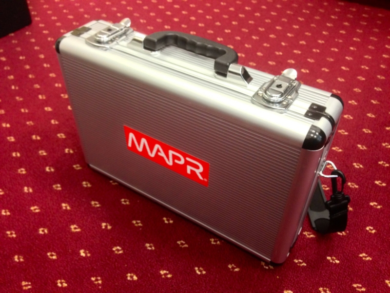
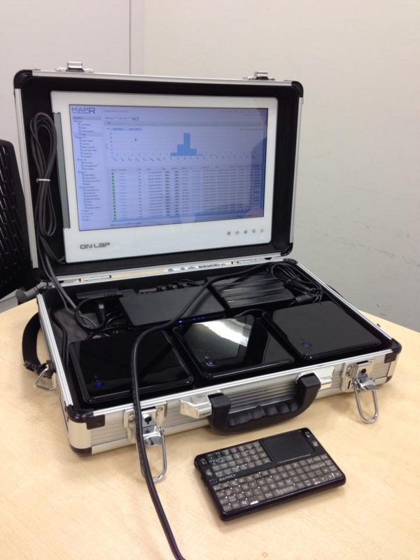
f:id:nagixx:20140609161347j:plainf:id:nagixx:20140609162049j:plain

The specifications are as follows.

  • 3 boxes of Intel NUC core i3 + 16GB memory + 128GB SSD
  • Gigabit Ethernet + IEEE 802.11na Wifi router
  • 13.3 inch HDMI-connected LCD monitor
  • 2.4GHz wireless keyboard + touchpad
  • A single power plug for the entire system
  • CentOS 6.6 + MapR M7 4.0.1 + CDH 5.3

Since each node has 16GB memory, most of applications work without any problem. I usually bring the cluster to meeting rooms and show demos to my customers. It is really useful because I can start the demos in one or two minutes if only one power outlet is available. A wifi connection is also available, so you I show the demos with a large screen using a LCD projector by accessing it from your laptop.

I have built this for Hadoop, but it can be used for any distributed software systems. For example, you can definitely use it as a demo system for MongoDB, Cassandra, Redis, Riak, Solr, Elasticsearch, Spark, Storm and so on. In fact, I run HP Vertica and Elasticsearch together with MapR in this portable cluster since MapR's NFS feature enables easy integration with any native applications.

The full parts list and how to build are shown below. Let's make your original one!

Parts List

The following parts list is as of June 10, 2014 including price information. This article is written based on the cluster built using those parts.

No.Part DescriptionUnit PriceAmount
01 Intel DC3217IYE (NUC barebone kit) 38,454 JPY 3
02 PLEXTOR PX-128M5M (128MB mSATA SSD) 14,319 JPY 3
03 CFD W3N1600Q-8G (8GB DDR3-1600 SO-DIMM x 2) 17,244 JPY 3
04 ELECOM LD-GPS/BK03 (0.3m CAT6 Gigabit LAN cable) 211 JPY 3
05 Miyoshi MBA-2P3 (Power cable 2-pin/3-pin conversion adapter) 402 JPY 3
06 FILCO FCC3M-04 (3-way splitter power cable) 988 JPY 1
07 Logitec LAN-W300N/IGRB (Gigabit/11na wifi router) 5,500 JPY 1
08 SANWA SUPPLY KB-DM2L (0.2m Power cable) 600 JPY 1
09 GeChic On-LAP 1302/J (13.3 inch LCD) 18,471 JPY 1
10 ELECOM T-FLC01-2220BK (2m Power cable) 639 JPY 1
11 EAPPLY EBO-013 (2.4GHz Wireless keyboard) 2,654 JPY 1
12 IRIS OYAMA AM-10 (Aluminum attache case) 2,234 JPY 1
13 Inoac A8-101BK (Polyethylene foam 10x1000x1000) 2,018 JPY 1
14 Kuraray 15RN Black (Velcro tape 25mm x 15cm) 278 JPY 2
15 Cemedine AX-038 Super X Clear (Versatile adhesive 20ml) 343 JPY 1

Half a year later, some parts are no longer sold in store, so I created a new list as of December 29, 2014. Currently, it will cost about 230,000 JPY in total. Note that some descriptions about component location or configuration may need to be updated. In particular, the NUC box was replaced with its successor model D34010WYK, which requires 1.35V low voltage memory and has a mini HDMI and a mini DisplayPort instead of a HDMI port. For this reason, the models of the memory and the LCD have also changed.

I'm using the wireless keyboard shown as No. 11 on the list, which I happened to have, but it is probably difficult to find one now. In that case, you can use Rii mini X1 or iClever IC-RF01 as an alternative. The reason I chose a device with 2.4GHz wireless technology rather than with Bluetooth is that it is recognized as a USB legacy device and can be used for the BIOS settings on boot.

No.Part DescriptionUnit PriceAmount
01 Intel D34010WYK (NUC barebone kit) 35,633 JPY 3
02 Transcend TS128GMSA370 (128MB mSATA SSD) 7,980 JPY 3
03 CFD W3N1600PS-L8G (8GB DDR3-1600 SO-DIMM x 2) 18,153 JPY 3
04 ELECOM LD-GPS/BK03 (0.3m CAT6 Gigabit LAN cable) 406 JPY 3
05 Diatec YL-3114 (Power cable 2-pin/3-pin conversion adapter) 494 JPY 3
06 FILCO FCC3M-04 (3-way splitter power cable) 1,008 JPY 1
07 Logitec LAN-W300N/IGRB (Gigabit/11na Wifi router) 6,000 JPY 1
08 SANWA SUPPLY KB-DM2L (0.2m Power cable) 429 JPY 1
09 GeChic On-LAP 1302 for Mac/J (13.3 inch LCD) 20,153 JPY 1
10 ELECOM T-FLC01-2220BK (2m Power cable) 994 JPY 1
11 Rii mini X1 (2.4GHz Wireless keyboard) 2,860 JPY 1
12 IRIS OYAMA AM-10 (Aluminum attache case) 2,271 JPY 1
13 Inoac A8-101BK (Polyethylene foam 10x1000x1000) 2,018 JPY 1
14 Kuraray 15RN Black (Velcro tape 25mm x 15cm) 270 JPY 2
15 Cemedine AX-038 Super X Clear (Versatile adhesive 20ml) 343 JPY 1

Assembling Bereborn Kits

It is quite easy to assemble NUC bareborn kits. Machines can be completed simply by installing memory and SSD.

First, when you loosen the screws at the four corners of the bottom panel and uncover it, you will see two SO-DIMM slots (on the left in the picture below) and two mini PCI Express slots (on the right in the picture).
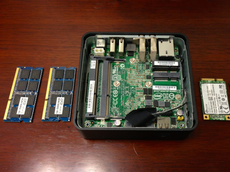
f:id:nagixx:20140421091249j:plain

Insert two memory modules into SO-DIMM slots, and fix them until they get locked into the latches. Out of the two mini PCI Express slots, the lower slot is for the half-size wireless LAN module, and the upper slot is for the full-size mSATA compliant slot. A wireless LAN module is not used this time, so just insert an mSATA SSD into the upper slot and screw it down.
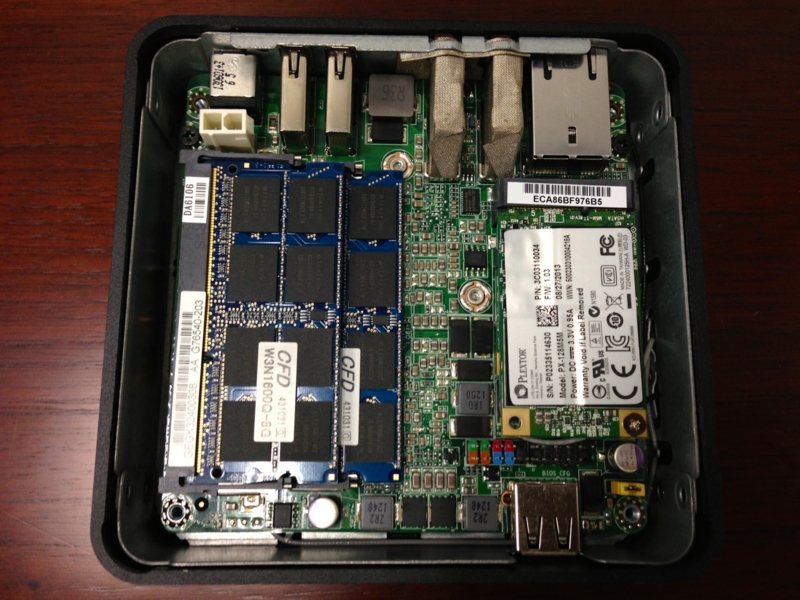
f:id:nagixx:20140421092516j:plain

After that, attach the bottom panel again and screw it down to complete the box.

Cutting Out the Cushioning Foam for the Aluminum Case

In order to pack three machines, AC adapters, a Wifi router, a LCD monitor and cables into this small case, they are required to be suitably arranged. In addition, they need to be securely fastened not to be moved when carrying the case around.

First, cut a 1cm-thick polyethylene foam sheet using a utility knife as pictured below. I chose a 15 times expansion polyethylene foam called PE-light A8, which is firm enough, because it is supposed to be used as a cushioning foam to hold relatively heavy parts.
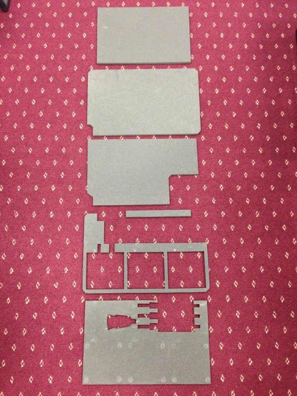
f:id:nagixx:20140123123824j:plain

Next, attach the first layer on the bottom of the case and the second layer on top of it. This will act as a frame to hold three machines, AC adapters and cables.

I used Cemedine Super X Clear for the adhesion of the polyethylene foam sheets. Basically, polyethylene is a hard-to-bond material, but this sheet is textured and Super X is an elastic adhesive with flexibility, so there is no problem in adhesive property.
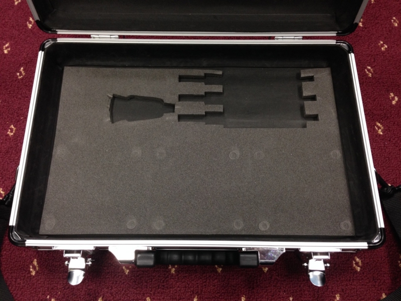
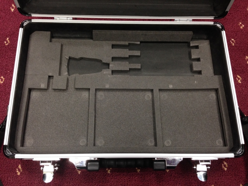
f:id:nagixx:20140123123933j:plainf:id:nagixx:20140123124057j:plain

On the upper side, velcro tapes are attached to secure a LCD monitor. These velcro tapes are self-adhesive but not strong enough to be attached to the surface of the cushioning foam on the upper side, so an adhesive bond is used.
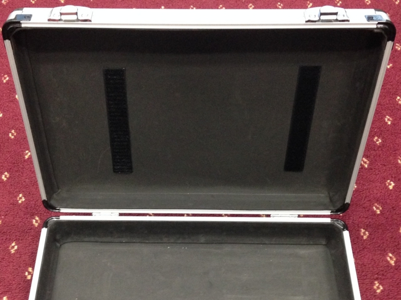
f:id:nagixx:20140123123555j:plain

The corresponding velcro tapes are also attached to the back of the LCD monitor. It is smooth-faced in contrast, therefore the tapes can be put directly on it.

This LCD, GeChic On-LAP, is a product which is supposed to be attached to the back of a laptop PC and used as a secondary monitor, but I chose it because it is very thin and runs on USB bus power. The mounting hardware for attachment to a laptop is removed since it is unnecessary this time.
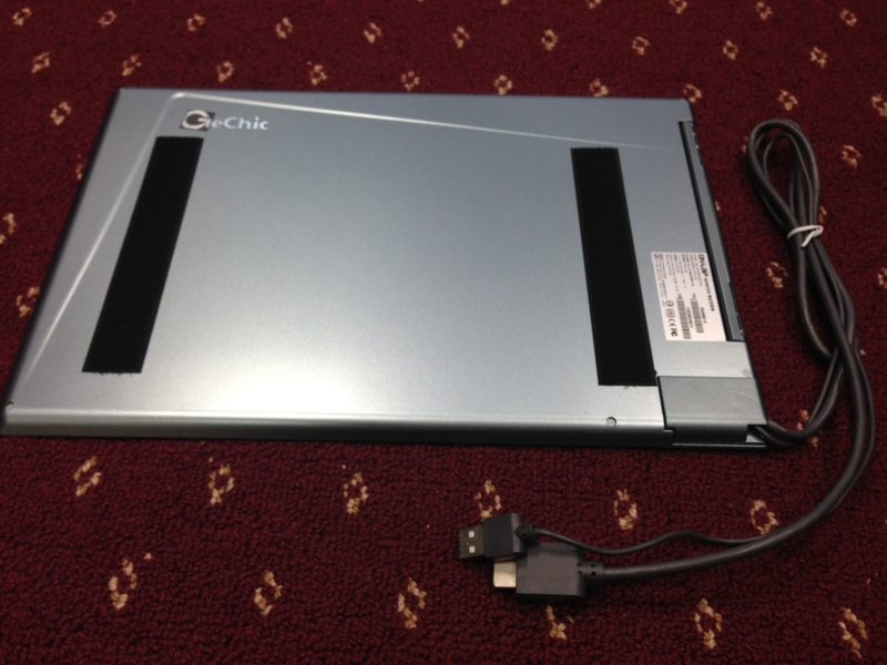
f:id:nagixx:20140123124354j:plain

In addition, three layers of the sheets are glued together to form the cushioning pad that covers LCD monitor to protect its surface as well as holds machines and cables when the case is closed.

The picture below is the LCD monitor (upper) side. The cutout in the bottom right corner is a space for monitor cables.

f:id:nagixx:20140123151513j:plain

Turning it over, you will see the machine (lower) side. The cutout of the double layer depth in the center is a storage space for a keyboard, and that of single layer depth at the bottom right is for a power plug.
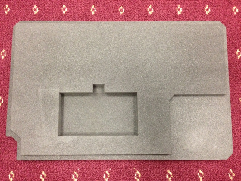
f:id:nagixx:20140611165340j:plain

By the way, for those who don't want to struggle to measure and cut those complex shapes, the drawing is ready for download as a PDF.
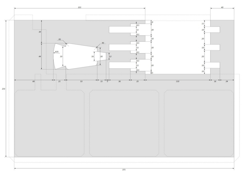
f:id:nagixx:20140611121500j:plain

Link to the PDF of the drawing

Layout of Components and Wiring

Arrange all the components step by step. Place three machines, put the AC adapters side by side and bind cables compactly. Since NUC's AC adapter has a 3-pin plug, they are connected via the 3-pin-to-2-pin conversion adapters to the 3 way splitter cable, and finally connected to the 2-way power strip. Then, the HDMI cable and the USB cable for power supply from the LCD monitor are plugged to the leftmost machine. The USB dongle for the wireless keyboard is also plugged into it.
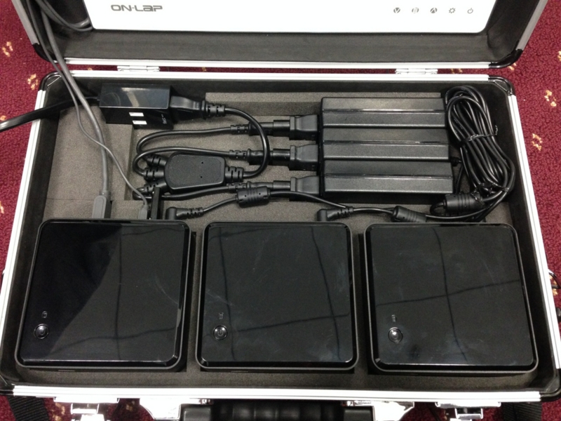
f:id:nagixx:20140123143455j:plain

Next, plug the L-type 2-pin power plug into the Wifi router and the other end into the remaining outlet of the power strip. And, connect the Ethernet port on each machine and the LAN-side port of the router using a LAN cable. The Wifi router is not fixed in place, but it fits into the space above the power split cable. There is no other Wifi router out in the market like this small-sized, self-powered Gigabit Ethernet router, so I was afraid of its end of sale... actually, it has already reached the end of sale. If you want to make this, find and get it as soon as possible!
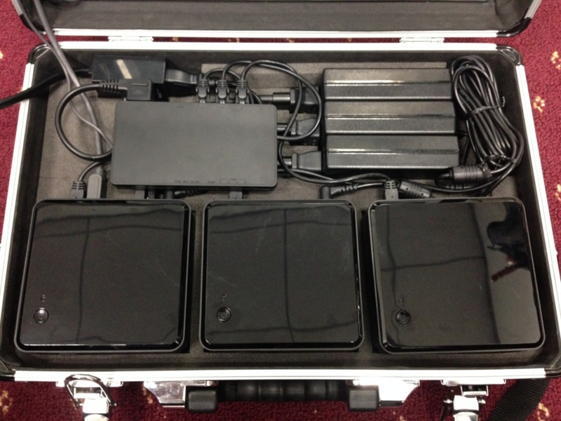
f:id:nagixx:20140123151704j:plain

These are all the steps to assemble the system. Now put the cushioning pad on top of the LCD monitor and place the keyboard in it. The power strip cable needs to be laid out about two rounds along the edge of the case, and place the plug to the location as shown below. By arranging this way, the cushioning forms tightly hold the machines and cables and they will never be moved around once the case is closed.
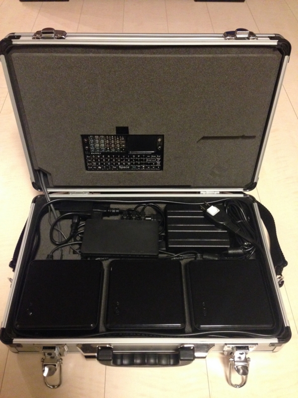
f:id:nagixx:20140124004724j:plain

Wifi Router Configuration

Before installing the OS, configure the Wifi router to get the network environment ready. First, plug the power cable into a wall outlet to turn the Wifi router on. The default SSID and pre-shared key for Wifi connection are described on the wireless encryption key sticker included in the product package, so enter them to establish a connection. The default IP address for the Wifi router is '192.168.2.1'. Open a web browser, go to 'http://192.168.2.1' and login with user name 'admin', password 'admin'.

In the administration screen, edit the following settings for the Portable Hadoop Cluster, and leave everything else as default. The SSID and pre-shared key can be any values you like. Regarding IP address for the cluster, use the default subnet of 192.168.2.0/24, but change the IP address of the router to 192.168.2.254, reserve 192.168.2.1 to 192.168.2.9 for the cluster nodes and other purpose as fixed addresses, and assign the remaining 192.168.2.10 to 192.168.2.253 for DHCP.

Menu CategoryMenu ItemItemValue
Wireless Settings Basic Settings SSID mapr-demo
Multi SSID Uncheck 'Valid' to disable it
Security Settings Shared Key Any passphrase
Wired Settings LAN-Side Settings Device's IP Address 192.168.2.254
Default Gateway 192.168.2.254
DHCP Client Range 192.168.2.10 - 192.168.2.253

Click 'Apply' button after completion of editing, then the Wifi router will restart. Lastly, plug the network cable with Internet access into the WAN-side port of the router, and move on to the next step.

CentOS Installation

The next step is software installation and configuration. Since NUCs have no DVD drive, use a USB flash drive for booting and perform network installation. Use a Windows PC to create a bootable image for installation on a USB flash drive.

First, download UNetbootin for Windows and CentOS 6.6 minimal image to a Windows PC.

Plug a USB flush drive into the Windows PC and launch UNetbootin. Select 'Diskimage' and specify CentOS-6.6-x86_64-minimal.iso that was downloaded in the previous step. Select 'USB Drive' in the Type field, specify the USB flush drive in the Drive field, and then click 'OK'. It takes a while to finish the process, and eject the USB flush drive when the boot image is created.

Next, install the OS on each machine. Since a monitor and keyboard are required, set up one by one by plugging the HDMI cable and the USB dongle for the wireless keyboard in and out.

Plug the USB flash drive into a NUC, and press the power button on the top panel to boot the machine. I only remember vaguely, but the USB flash drive should be recognized as a boot device because the SSD is empty, and installation process will start. (If it doesn't start, hold F2 key during boot-up and select the USB flash drive in the [Boot] menu.)

I'm not going into detail about the CentOS installation process, but I will list a few important points as follows.

  • In the 'Installation Method' screen, select 'URL' as an installation media type. In the 'Configure TCP/IP' screen, proceed with the default settings of DHCP. In the 'URL Setup' screen, enter 'http://ftp.riken.jp/Linux/centos/6/os/x86_64/' in the topmost field.
  • In the host name setting screen, enter the host name 'node1', 'node2' and 'node3', respectively from left to right. In addition, click the 'Configure Network' button at the bottom left of the same screen, select the device 'System eth0' in the 'Wired' tab and go to 'Edit'. Select 'Manual' in the Method drop down menu in the 'IPv4 Settings' tab. Add the address '192.168.2.1', '192.168.2.2' and '192.168.2.3', respectively from left to right, with the netmask '24' and the gateway '192.168.2.254', and enter the DNS server '192.168.2.254'.
  • In the installation type selection screen, select 'Create Custom Layout' and create the layout as follows in the partition edit screen. Assign standard partitions and don't use LVM.
    DeviceSizeMount PointType
    /dev/sda1 200MB /boot/efi EFI
    /dev/sda2 200MB /boot ext4
    /dev/sda3 58804MB / ext4
    /dev/sda4 58804MB /mapr ext4
    /dev/sda5 4095MB   swap
  • In the installation software selection screen, select 'Desktop'.

When the installation completes, machines will restart. In the post installation setup screen after restart, 'Create User' is unnecessary for the moment, so proceed with blank. In the 'Date and Time', check 'Synchronize date and time over the network'. 'Kdump' is unnecessary. These are all the steps to setup the OS.

Miscellaneous OS Configuration

As a preparation for building the Hadoop Cluster, make miscellaneous OS configuration settings. Perform the following steps on each node.

Edit '/etc/sysconfig/i18n' as follows to set the system language to 'en_US.UTF-8'.

LANG="en_US.UTF-8"

Edit the following line in '/etc/sysconfig/selinux' to disable SELinux.

SELINUX=disabled

Now, restart the machine. This will disable SELinux, but some files are still labeled with a SELinux context, so delete such information with the following command.

# find / -print0 | xargs -r0 setfattr -x security.selinux 2>/dev/null

Add the following lines to '/etc/sysctl.conf'.

vm.overcommit_memory=0
net.ipv4.tcp_retries2=5

Run the following command to reflect the changes.

# sysctl -p

Edit '/etc/hosts' as follows.

127.0.0.1       localhost
192.168.2.1 node1
192.168.2.2 node2
192.168.2.3 node3

Run the following commands to stop the iptables services and disable them on startup.

# service iptables stop
# service ip6tables stop
# chkconfig iptables off
# chkconfig ip6tables off

Edit '/etc/ntp.conf' to configure NTP so that the clocks of three nodes are synchronized. The factory default settings are to synchronize with the NTP servers on the Internet. However, this Portable Hadoop Cluster doesn't always have the Internet connection, so configure every node to be synchronized with a local clock on node1.

On node1, edit the following lines in '/etc/ntp.conf'. Comment out the default server setting, and specify '127.127.1.0', which stands for host's local clock.

nrestrict 192.168.2.0 mask 255.255.255.0 nomodify notrap
server 127.127.1.0
#server 0.centos.pool.ntp.org
#server 1.centos.pool.ntp.org
#server 2.centos.pool.ntp.org

On node2 and node3, edit the following lines in '/etc/ntp.conf'. The reference source is set to node1.

server node1
#server 0.centos.pool.ntp.org
#server 1.centos.pool.ntp.org
#server 2.centos.pool.ntp.org

Restart the NTP service with the following command.

# service ntpd restart

Create the MapR system user and group with the following commands. Set the password of your choice.

# groupadd mapr -g 500
# useradd mapr -u 500 -g 500
# passwd mapr

It is convenient if the root user and the mapr user can login to other nodes via ssh without password. The following commands set up a password-less ssh login.

# ssh-keygen -t rsa -N '' -f ~/.ssh/id_rsa
# for host in node1 node2 node3; do ssh-copy-id $host; done
# su - mapr
$ ssh-keygen -t rsa -N '' -f ~/.ssh/id_rsa
$ for host in node1 node2 node3; do ssh-copy-id $host; done
$ exit

Install OpenJDK from the yum repository with the following command.

# yum install java-1.7.0-openjdk-devel

In the installation process, the partition '/dev/sda4' was created for MapR and mounted on '/mapr'. Since MapR accesses block devices directly, unmount this file system.

# umount /mapr

In addition, edit '/etc/fstab' to remove the line of /dev/sda4 so as not to be mounted on startup.

MapR Installation

The last step is the installation of the MapR distribution for Hadoop. Perform the following steps on each node.

First, create '/etc/yum.repos.d/maprtech.repo' to configure the MapR yum repository.

[maprtech]
name=MapR Technologies
baseurl=http://package.mapr.com/releases/v4.0.1/redhat/
enabled=1
gpgcheck=0
protect=1

[maprecosystem]
name=MapR Technologies
baseurl=http://package.mapr.com/releases/ecosystem-4.x/redhat
enabled=1
gpgcheck=0
protect=1

Since some EPEL packages are also required, run the following commands to configure the EPEL repository.

# wget http://download.fedoraproject.org/pub/epel/6/x86_64/epel-release-6-8.noarch.rpm
# yum localinstall epel-release-6-8.noarch.rpm

Next, install MapR packages. For MapR 4.x, both MapReduce v1 and v2 (YARN) applications can run at the same time, but they can not share the same memory space. So, select either v1 or v2 for this cluster to use a limited 16GB memory efficiently.

Run the following commands for the MapReduce v1 configuration.

# yum install mapr-cldb mapr-core mapr-core-internal mapr-fileserver \
mapr-hadoop-core mapr-jobtracker mapr-mapreduce1 mapr-nfs mapr-tasktracker \
mapr-webserver mapr-zk-internal mapr-zookeeper

Run the following commands for the MapReduce v2 configuration. Since the History Server can be configured only on a single node, the mapr-historyserver package is installed only on node1.

# yum install mapr-cldb mapr-core mapr-core-internal mapr-fileserver \
mapr-hadoop-core mapr-historyserver mapr-mapreduce2 mapr-nfs mapr-nodemanager \
mapr-resourcemanager mapr-webserver mapr-zk-internal mapr-zookeeper

The following command will create the file that specifies the partition for the MapR data.

# echo "/dev/sda4" > disks.txt

The following command will perform initialization and configuration of MapR. After running this command, the appropriate services will start automatically. For MapReduce v1 configuration:

# /opt/mapr/server/configure.sh -N cluster1 -C node1,node2,node3 \
-Z node1,node2,node3 -F disks.txt

For MapReduce v2 configuration:

# /opt/mapr/server/configure.sh -N cluster1 -C node1,node2,node3 \
-Z node1,node2,node3 -RM node1,node2,node3 -HS node1 -F disks.txt

Once these configurations have been completed on all the three nodes, the MapR cluster will become active in a few minutes. However, there is the issue in MapR 4.0.1 that users of some browser may lose the ability to access MapR via HTTPS because recent version of them have removed support for older certificate cipher algorithms. Run the following commands on each node to install the patch for this issue. The last command will restart the Web servers, and the web interface will become active in a few minutes.

# wget http://package.mapr.com/scripts/mcs/fixssl
# chmod 755 fixssl
# ./fixssl

Open a web browser and go to 'http://192.168.2.1:8443', then the MapR Control System screen will be shown. Login to it with the user name 'mapr' and the password that you have set when creating the user.
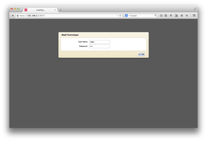
f:id:nagixx:20141230001615p:plain

f:id:nagixx:20141230001642p:plain

Register the MapR cluster via Web and obtain a license key. By factory default, a Base License is applied, but if a free perpetual M3 license or a free 30-day trial M5 license is applied, the NFS access, high-availability and data management features such as snapshot will be enabled.

Click 'Manage Licenses' at the top right of the MapR Control System screen, and click 'Add Licenses via Web' button in the dialog appeared. You will be asked if going to MapR's web site, then click 'OK' to proceed. Once a form for user registration is filled out and submitted on the web site, select either a M3 or M5 license, and a license will be published. Go back to the MapR Control System screen, and click 'Add Licenses via Web' button in 'Manage Licenses' dialog to apply the obtained license.

Now, run a sample MapReduce job. This is a sample MapReduce job which calculates pi. For MapReduce v1:

$ hadoop -classic jar /opt/mapr/hadoop/hadoop-0.20.2/hadoop-0.20.2-dev-examples.jar pi 10 10000

For MapReduce v2:

$ hadoop -yarn jar /opt/mapr/hadoop/hadoop-2.4.1/share/hadoop/mapreduce/hadoop-mapreduce-examples-2.4.1-mapr-1408.jar pi 10 10000

Lastly, add the settings that are specific to this Portable Hadoop Cluster. In the MapR's default configuration, relatively large memory is assigned to each MapR daemon process, but the machines in this cluster have a relatively small, 16GB memory, so edit the following lines in '/opt/mapr/conf/warden.conf' on each node to minimize the memory assigned so that much more memory will be assigned to MapReduce jobs.

service.command.jt.heapsize.max=256
service.command.tt.heapsize.max=64
service.command.cldb.heapsize.max=256
service.command.mfs.heapsize.max=4000
service.command.webserver.heapsize.max=512
service.command.nfs.heapsize.max=64
service.command.os.heapsize.max=256
service.command.warden.heapsize.max=64
service.command.zk.heapsize.max=256

For MapReduce v2 configuration, edit the following files in addition to the above.

/opt/mapr/conf/conf.d/warden.resourcemanager.conf

service.heapsize.max=256

/opt/mapr/conf/conf.d/warden.nodemanager.conf

service.heapsize.max=64

/opt/mapr/conf/conf.d/warden.historyserver.conf

service.heapsize.max=64

After completing the steps above, run the following command on each node to restart services so as to reflect the changes.

# service mapr-warden restart

Extra tips

Login Screen Resolution Settings

When the machine starts up, the screen of the leftmost machine node1 will appear on the LDC, but it is a bit blurred because the resolution of the login screen is not identical to that of LCD. In order to adjust it, run the following command to check the connected monitor name. In this case, it is 'HDMI-1'.

# xrandr -q
Screen 0: minimum 320 x 200, current 1366 x 768, maximum 8192 x 8192
VGA-0 disconnected (normal left inverted right x axis y axis)
HDMI-0 disconnected (normal left inverted right x axis y axis)
DP-0 disconnected (normal left inverted right x axis y axis)
HDMI-1 connected 1366x768+0+0 (normal left inverted right x axis y axis) 460mm x 270mm
1366x768 59.8*
1024x768 75.1 70.1 60.0
800x600 75.0 60.3
640x480 75.0 60.0
DP-1 disconnected (normal left inverted right x axis y axis)

Then, edit '/etc/X11/xorg.conf.d/40-monitor.conf' as follows.

Section "Monitor"
Identifier "HDMI-1"
Option "PreferredMode" "1366x768"
EndSection

Auto Login

When doing a demo using this cluster, it is convenient if one can automatically login and move on from the login screen to the desktop screen without interaction. If you like, edit '/etc/gdm/custom.conf' as follows. In this case, an automatic login will be performed as the mapr user after waiting for user input for 30 seconds.

[daemon]
TimedLoginEnable=true
TimedLogin=mapr
TimedLoginDelay=30

Shutdown Via Power Button

When shutting down the portable cluster, it is convenient as well if one can power off the machines without entering a password or click a button for confirmation but just by pressing the power button on the top panel of the NUCs. Edit '/etc/polkit-1/localauthority.conf.d/org.freedesktop.logind.policy' as follows to enable it.

<?xml version="1.0" encoding="UTF-8"?>
<!DOCTYPE policyconfig PUBLIC
"-//freedesktop//DTD PolicyKit Policy Configuration 1.0//EN"
"http://www.freedesktop.org/standards/PolicyKit/1.0/policyconfig.dtd">
<policyconfig>
<action id="org.freedesktop.login1.power-off-multiple-sessions">
<description>Shutdown the system when multiple users are logged in</description>
<message>System policy prevents shutting down the system when other users are logged in</message>
<defaults>
<allow_inactive>yes</allow_inactive>
<allow_active>yes</allow_active>
</defaults>
</action>
</policyconfig>

図解 MapR のメモリ管理

MapR Hadoopディストリビューションにおいて、メモリがどのように割り当てられているかは一見わかりにくいので、図を使いながら詳細を解説していきましょう。なお、説明はMapR 5.0のYARN構成がベースになっています。YARNアプリケーションのメモリ割り当ての説明以降は、どのHadoopディストリビューションでも同じなので広く参考になると思います。

MapRのサービスのメモリ割り当て

MapRでは各ノードで管理や処理を担うプロセスを「サービス」として定義しています。一般的なHadoopにも存在するYARNのResourceManagerやNodeManagerといったサービスもあれば、HDFSの代わりにファイルシステムの機能を提供するMapR-FSやCLDBのようなサービスや、NFSサーバ機能を提供するNFSサービス、Web UI機能を提供するMapR Control Systemサービスなどが存在します。

その中で、すべてのサービスのライフサイクルを管理する役割を提供するWardenというサービスがあります。いわばサービスをまとめて管理するサービスです。Wardenサービスの重要な役割の一つに、各サービスにどれだけメモリリソースを割り当てるかを管理する機能があります。

Wardenはクラスタ起動時に物理メモリ容量を取得し、設定ファイルをもとに各サービスが利用可能なメモリ容量を計算し、サービスごとに割り当てていきます。設定ファイルの一つ/opt/mapr/conf/warden.confを見ながら、例としてZooKeeperサービスに割り当てられるメモリがどのように計算されるかを見ていきます。

service.command.zk.heapsize.percent=1
service.command.zk.heapsize.max=1500
service.command.zk.heapsize.min=256

上記はZooKeeperのメモリ割り当てを記述している部分ですが、原則としてノードの物理メモリに対するpercentの割合がそのサービスに割り当てられます。ただし、上限としてmax、下限としてminの値が決められていますので、その範囲を外れる場合は上限または下限に値が調整されます。

例として、物理メモリがそれぞれ192GB、64GB、16GBの3つのパターンについて見てみましょう。

f:id:nagixx:20150811181052p:plain

物理メモリが64GBのノードの場合は64GB×1%=655MBがZooKeeperに割り当てられます。一方、192GBのノードの場合は192GB×1%=1966MBになりますが、これは上限の1500MBを超えていますので、割り当て値は1500MBになります。同様に、16GBのノードの場合は16GB×1%=164MBで下限を下回るため、割り当て値は256MBになります。

上記の計算がすべてのサービスに対して適用されます。ノードによってインストールされるサービスが異なるため、各ノードでのメモリ割り当ても異なる結果になります。

MapR 特有のコアサービスに関しての設定は/opt/mapr/conf/warden.confファイルに記述されています。この中に、OSに割り当てるメモリの設定があります。この項目は実際にはサービスではありませんが、OSの稼働に必要なメモリ容量は計算上確保しておく必要があるため存在しています。また、MapR-FSサービスの設定には割合と下限の項目はありますが、上限はありません。

以下に、パラメータとデフォルト値の一覧を示します。

/opt/mapr/conf/warden.conf

パラメータデフォルト値説明
service.command.cldb.heapsize.percent 8 CLDBに割り当てる物理メモリの割合(%)
service.command.cldb.heapsize.max 4000 CLDBが利用可能な最大メモリ容量(MB)
service.command.cldb.heapsize.min 256 CLDBが最低限確保するメモリ容量(MB)
service.command.mfs.heapsize.percent 35 MapR-FSに割り当てる物理メモリの割合(%)
service.command.mfs.heapsize.maxpercent 85 余剰メモリ容量がある場合にMapR-FSが利用可能な最大の物理メモリの割合(%)。YARN環境では使われない
service.command.mfs.heapsize.max 512 MapR-FSが最低限確保するメモリ容量(MB)
service.command.webserver.heapsize.percent 3 MapR Control Systemに割り当てる物理メモリの割合(%)
service.command.webserver.heapsize.max 750 MapR Control Systemが利用可能な最大メモリ容量(MB)
service.command.webserver.heapsize.min 512 MapR Control Systemが最低限確保するメモリ容量(MB)
service.command.nfs.heapsize.percent 3 NFSに割り当てる物理メモリの割合(%)
service.command.nfs.heapsize.max 1000 NFSが利用可能な最大メモリ容量(MB)
service.command.nfs.heapsize.min 64 NFSが最低限確保するメモリ容量(MB)
service.command.os.heapsize.percent 10 OSに割り当てる物理メモリの割合(%)
service.command.os.heapsize.max 4000 OSが利用可能な最大メモリ容量(MB)
service.command.os.heapsize.min 256 OSが最低限確保するメモリ容量(MB)
service.command.warden.heapsize.percent 1 Wardenに割り当てる物理メモリの割合(%)
service.command.warden.heapsize.max 750 Wardenが利用可能な最大メモリ容量(MB)
service.command.warden.heapsize.min 64 Wardenが最低限確保するメモリ容量(MB)
service.command.zk.heapsize.percent 1 ZooKeeperに割り当てる物理メモリの割合(%)
service.command.zk.heapsize.max 1500 ZooKeeperが利用可能な最大メモリ容量(MB)
service.command.zk.heapsize.min 256 ZooKeeperが最低限確保するメモリ容量(MB)

YARNコンポーネントのサービスやHadoopエコシステムのサービスに関しては、/opt/mapr/conf/conf.d/ディレクトリ以下のwarden.<サービス名>.confという名前の、サービスごとの個別ファイルに設定があります。MapRコアサービスとは異なり、メモリ割り当てのデフォルト値は記載されていません。ノード上のメモリ割り当てを厳密に管理したい場合には、明示的に下記のパラメータを指定する必要があります。

/opt/mapr/conf/conf.d/warden.<サービス名>.conf

パラメータ説明
service.heapsize.percent サービスに割り当てる物理メモリの割合(%)
service.heapsize.max サービスが利用可能な最大メモリ容量(MB)
service.heapsize.min サービスが最低限確保するメモリ容量(MB)

サービス名と対応するパッケージ名は下表を参照してください。

サービス名説明パッケージ名
drill-bits Drillサービス mapr-drill
gateway MapR Gatewayサービス mapr-gateway
hue Hueサービス mapr-hue
httpfs HttpFSサービス mapr-httpfs
hbasethrift HBase Thriftサービス mapr-hbasethrift
hbase-rest HBase REST Gatewayサービス mapr-hbase-rest
historyserver YARN Job History Serverサービス mapr-historyserver
hivemeta Hive Metastoreサービス mapr-hivemetastore
hs2 HiveServer2サービス mapr-hiveserver2
nodemanager YARN Node Managerサービス mapr-nodemanager
oozie Oozieサービス mapr-oozie
resourcemanager YARN Resource Managerサービス mapr-resourcemanager
spark-master Spark Masterサービス mapr-spark-master

MapRサービス用メモリの積み上げ

このように各サービスで個別に計算した割り当てメモリサイズを積み上げて、サービス用割り当て容量の合計サイズが求められます。

ここで、CLDBおよびZooKeeperサービスが稼働するノードのみに適用する例外があります。もしどちらかのサービスがそのノードに構成されていると、1500MB(ただしサービス用割り当て容量の合計が6GB未満であれば、その25%)がマージンとして確保されます。これは、CLDBまたはZooKeeperはクラスタの稼働のための重要なプロセスであり、万が一にもメモリ不足による停止もしくは応答の中断が発生することを避け、余裕を持たせるためです。

さて、物理メモリ容量から、サービス用割り当て容量とCLDB/ZooKeeper用のマージンを差し引いた残りは、YARNアプリケーションに提供されることになります。一般的なHadoopでは、YARNアプリケーション用のメモリサイズはパラメータyarn.nodemanager.resource.memory-mb (yarn-site.xml)にてあらかじめ定義しておく必要がありますが、MapRの場合は上記の通りWardenが計算した結果が、yarn.nodemanager.resource.memory-mbパラメータとしてYARN NodeManagerに自動的に引き渡されます。

f:id:nagixx:20150811185740p:plain

具体的な計算例を見ていきましょう。64GB (=65536MB)の物理メモリを搭載したマシンがある場合、各サービスに割り当てられるメモリは次の通りになります。

サービス名percentminmax計算結果
cldb 8 256 4000 4000
mfs 35 512 - 22937
webserver 3 512 750 750
nfs 3 64 1000 1000
os 10 256 4000 4000
warden 1 64 750 655
zk 1 256 1500 655
サービス合計 33997
cldb/zkマージン 1500
YARNアプリケーション用メモリ 30039

この場合、30039MBがYARNアプリケーションに割り当てられることになります。

MapRサービスで実際に使われるメモリ容量

ところで、Wardenで計算されたサービスのメモリ割り当ては、実際に使用されるメモリ容量に反映されるのでしょうか。実は、Wardenの設定がサービス起動時にプロセスに反映されるサービスと、反映されないサービスの2通りがあります。

例えばMapR-FSサービスは、Warden設定から計算された割り当て容量がMapR-FSプロセスに渡され、実際にOSのコマンドで確認すると設定されたサイズでメモリが確保されていることがわかります。一方、NodeManagerサービスは、Warden設定が計算上利用されますが、JVM起動時の最大ヒープサイズの指定にはyarn-env.shの環境変数YARN_NODEMANAGER_HEAPSIZEが使用されます。

ということで、実際に使われるメモリ容量が指定されているプロパティを表としてまとめました。ちなみにJVMで動作するサービスの場合、指定されたメモリ容量がJVMの最大ヒープサイズとして設定されますが、JVMはメモリが必要になったときに初めて物理メモリがマップされるため、常にすべての容量が確保されるわけではありません。念のため。

サービス名プロパティデフォルト値ファイル名
cldb Warden設定
mfs Warden設定
webserver Warden設定
nfs Warden設定
os 環境による
warden JVMのデフォルト値(物理メモリの1/4)
zk JVMのデフォルト値(物理メモリの1/4)
historyserver HADOOP_JOB_HISTORYSERVER_HEAPSIZE 1000 mapred-env.sh
nodemanager YARN_NODEMANAGER_HEAPSIZE 1000 yarn-env.sh
resourcemanager YARN_RESOURCEMANAGER_HEAPSIZE 1000 yarn-env.sh
drill DRILL_MAX_DIRECT_MEMORY 8G drill-env.sh
DRILL_HEAP 4G

YARNアプリケーションのメモリ割り当て

YARNアプリケーションに対するメモリ割り当てのしくみも結構込み入っているため、正確に把握している人は意外に少ないような気がします。YARNフレームワークは汎用的なリソース管理のしくみを持っていますが、YARN上で動作する代表的なアプリケーションの1つであるMapReduce (MRv2)を例として、メモリが割り当てられる流れを見ていきます。

関連するパラメータは以下の通りです。

/opt/mapr/hadoop/hadoop-2.7.0/etc/hadoop/yarn-site.xml

パラメータデフォルト値説明
yarn.nodemanager.resource.memory-mb Wardenによる計算 YARNコンテナに割り当てることのできるメモリ容量(MB)
yarn.scheduler.minimum-allocation-mb 1024 メモリ要求に対しYARNスケジューラが割り当てる最小メモリサイズ(MB)。CapacitySchedulerの場合、割り当てるメモリサイズの単位にもなる
yarn.scheduler.increment-allocation-mb 1024 (FairSchedulerのみ)メモリ要求に対しYARNスケジューラが割り当てるメモリサイズの単位(MB)
yarn.scheduler.maximum-allocation-mb 8192 メモリ要求に対しYARNスケジューラが割り当てる最大メモリサイズ(MB)

/opt/mapr/hadoop/hadoop-2.7.0/etc/hadoop/mapred-site.xml

パラメータデフォルト値説明
yarn.app.mapreduce.am.resource.mb 1536 MRv2のApplicationMasterのコンテナのメモリサイズ(MB)
mapreduce.map.memory.mb 1024 MRv2のMap Taskのコンテナのメモリサイズ(MB)
mapreduce.reduce.memory.mb 3072 MRv2のReduce Taskのコンテナのメモリサイズ(MB)

NodeManagerが起動する際には、まずパラメータyarn.nodemanager.resource.memory-mbが利用できるメモリ容量として読み込まれます。前述の通り、MapRの場合はWardenが自動計算したサイズが使われます。

MRv2アプリケーションの実行時には、アプリケーションの処理を行うYARNコンテナに必要なメモリサイズが、ResourceManagerのYARNスケジューラに対して要求されます。MRv2のApplicationMasterを実行するコンテナのメモリサイズはyarn.app.mapreduce.am.resource.mb、Map Taskを実行するコンテナのメモリサイズはmapreduce.map.memory.mb、Reduce Taskを実行するコンテナのメモリサイズはmapreduce.reduce.memory.mbで指定された値が読み込まれ、要求が行われます。

f:id:nagixx:20150812094448p:plain

割り当てるメモリサイズはFairSchedulerの場合yarn.scheduler.increment-allocation-mb、CapacitySchedulerの場合yarn.scheduler.minimum-allocation-mbの倍数である必要があり、要求されたメモリサイズがこれらのパラメータのちょうど倍数になっていない場合には、要求を受けたYARNスケジューラは、最も近い倍数に繰り上げたサイズを割り当てます。また、メモリサイズが下限のyarn.scheduler.minimum-allocation-mbおよび上限のyarn.scheduler.maximum-allocation-mbで指定される範囲に収まっているかを確認し、範囲を外れる場合には上限または下限に値を調整します。これらは「リソースの正規化」と呼ばれます。

見方を変えると、yarn.app.mapreduce.am.resource.mb、mapreduce.map.memory.mb、mapreduce.reduce.memory.mbの値がyarn.scheduler.increment-allocation-mbやyarn.scheduler.minimum-allocation-mbの倍数になっていない場合には必要以上の容量がコンテナに割り当てられることになるため、メモリ利用効率を最大にするためにはこれらの倍数にあわせることが重要になります。

YARNスケジューラは、各ノードのNodeManagerが管理する利用可能なリソースの中から、上記の通り計算されたリソースをコンテナに割り当て、処理が実行されます。

YARNコンテナで実際に使われるメモリ容量

MapReduceアプリケーション用に設定するメモリ関連の項目には、他にも次のようなパラメータが存在します。これらはJVMで利用する最大ヒープサイズを指定していますが、なぜコンテナ用のメモリサイズとJVMの最大ヒープサイズの2種類の設定項目があるのでしょうか。 

/opt/mapr/hadoop/hadoop-2.7.0/etc/hadoop/mapred-site.xml

パラメータデフォルト値説明
yarn.app.mapreduce.am.command-opts -Xmx1024m MRv2のApplicationMasterのJVM最大ヒープサイズ
mapreduce.map.java.opts -Xmx900m MRv2のMap TaskのJVM最大ヒープサイズ
mapreduce.reduce.java.opts -Xmx2560m MRv2のReduce TaskのJVM最大ヒープサイズ

その理由は、JVMのヒープサイズはJVMの世代別GCで扱われる領域のうち、Eden、Survivor、Old領域のみを対象としており、それ以外に使われるメモリ容量は別に管理する必要があるためです。

それ以外に使用される可能性があるメモリとしては、Permanent領域(クラス/メソッド/static変数)、Cヒープ(JVM自体の内部使用メモリ)、スレッドスタック(メソッドの呼び出し階層情報/変数)、JNI呼び出しのネイティブコード、Forkされた子プロセスのメモリ、などがあります。これらが知らないうちにノード内のメモリを使い尽くしてしまうことを防ぐため、各ノードに存在するcontainer-executorというプロセスがYARNコンテナで利用されるメモリを管理・監視しています。JVM自体もcontainer-executorがForkする子プロセスであるため、container-executorはプロセスツリーをもとに使用メモリ容量を監視して、各コンテナに割り当てられたメモリサイズに収まっているかを確認し、超過していればJVMプロセスおよびその子プロセスを強制的に終了させます。

f:id:nagixx:20150812095125p:plain

では、コンテナ用のメモリサイズに対してJVMの最大ヒープサイズをどれくらいに設定しておけばよいか、ということですが、アプリケーションコードにも依存しますが、だいたいコンテナ用のメモリサイズの75〜80%程度にしておけば問題ないケースが多いです。

以上、YARNアプリケーションとしてMapReduceの例で説明をしましたが、TezやSparkなどでは異なるパラメータの設定があります。ただ、YARNスケジューラの部分の考え方は変わりませんので、参考にしていただければと思います。

政府統計情報 e-Stat を Apache Drill で分析してみる (3)

前回の記事からの続きです。

ビューを作成

前回までに、平成22年の国勢調査における人口増減に関する統計データを取得するところまでいきました。今回はSQLを使って統計データの集計をしていきます。

まずデータをSQLで扱いやすくするために、使用するデータはビューとして定義しておくことにします。 「CREATE VIEW」句を使用しますが、ビューの名前は「dfs.tmp.`ビュー名`」のようになっています。dfs.tmpはスキーマの名前で、ファイルシステムのテンポラリディレクトリにビューの定義ファイルが保存されることを意味しています。ここでは地域名を取り出すためのビューと、統計データを取り出すためのビューを定義します。

0: jdbc:drill:zk=local> CREATE VIEW dfs.tmp.`area_info` AS SELECT
. . . . . . . . . . . >   t.data.`@code` code,
. . . . . . . . . . . >   t.data.`@name` name,
. . . . . . . . . . . >   t.data.`@level` level,
. . . . . . . . . . . >   t.data.`@parentCode` parent
. . . . . . . . . . . > FROM (
. . . . . . . . . . . >   SELECT
. . . . . . . . . . . >     FLATTEN(f.GET_STATS_DATA.STATISTICAL_DATA.CLASS_INF.CLASS_OBJ[2].CLASS) data
. . . . . . . . . . . >   FROM
. . . . . . . . . . . >     dfs.`/tmp/stats_data_modified.json` f
. . . . . . . . . . . > ) t;
+-------+------------------------------------------------------------+
|  ok   |                          summary                           |
+-------+------------------------------------------------------------+
| true  | View 'area_info' created successfully in 'dfs.tmp' schema  |
+-------+------------------------------------------------------------+
1 row selected (0.103 seconds)
0: jdbc:drill:zk=local> CREATE VIEW dfs.tmp.`stats_data` AS SELECT
. . . . . . . . . . . >   t.data.`@tab` tab,
. . . . . . . . . . . >   t.data.`@cat01` did,
. . . . . . . . . . . >   t.data.`@area` area,
. . . . . . . . . . . >   t.data.$ val
. . . . . . . . . . . > FROM (
. . . . . . . . . . . >   SELECT
. . . . . . . . . . . >     FLATTEN(f.GET_STATS_DATA.STATISTICAL_DATA.DATA_INF.`VALUE`) data
. . . . . . . . . . . >   FROM
. . . . . . . . . . . >     dfs.`/tmp/stats_data_modified.json` f
. . . . . . . . . . . > ) t;
+-------+-------------------------------------------------------------+
|  ok   |                           summary                           |
+-------+-------------------------------------------------------------+
| true  | View 'stats_data' created successfully in 'dfs.tmp' schema  |
+-------+-------------------------------------------------------------+
1 row selected (0.155 seconds)

ビューの定義ファイルは/tmpに「.view.drill」という拡張子のついたJSONファイルとして保存されています。

$ ls /tmp
area_info.view.drill
stats_data_modified.view.drill

ビューの内容を確認してみます。

0: jdbc:drill:zk=local> SELECT * FROM dfs.tmp.`area_info` LIMIT 10;
+--------+--------+--------+---------+
|  code  |  name  | level  | parent  |
+--------+--------+--------+---------+
| 00000  | 全国     | 1      | null    |
| 00001  | 全国市部   | 1      | null    |
| 00002  | 全国郡部   | 1      | null    |
| 01000  | 北海道    | 2      | 00000   |
| 01001  | 北海道市部  | 3      | 01000   |
| 01002  | 北海道郡部  | 3      | 01000   |
| 01100  | 札幌市    | 3      | 01000   |
| 01101  | 中央区    | 4      | 01100   |
| 01102  | 北区     | 4      | 01100   |
| 01103  | 東区     | 4      | 01100   |
+--------+--------+--------+---------+
10 rows selected (11.902 seconds)
0: jdbc:drill:zk=local> SELECT * FROM dfs.tmp.`stats_data` LIMIT 10;
+------+--------+--------+------------+
| tab  |  did   |  area  |    val     |
+------+--------+--------+------------+
| 020  | 00710  | 00000  | 128057352  |
| 020  | 00710  | 00001  | 116156631  |
| 020  | 00710  | 00002  | 11900721   |
| 020  | 00710  | 01000  | 5506419    |
| 020  | 00710  | 01001  | 4449360    |
| 020  | 00710  | 01002  | 1057059    |
| 020  | 00710  | 01100  | 1913545    |
| 020  | 00710  | 01101  | 220189     |
| 020  | 00710  | 01102  | 278781     |
| 020  | 00710  | 01103  | 255873     |
+------+--------+--------+------------+
10 rows selected (87.308 seconds)

検索・集計する

さて、ここまで来たら、あとはもう普通のSQLです。まずは市区町村の人口増加率トップ10を出してみましょう。

下記のクエリの条件の部分では、表章項目コードが102(=人口)、人口集中地区区分を表すDIDコードが00710(=全域)、値が「-」(=無効)ではないレコードを取り出しています。また、ソートをする際には値をDOUBLE型にキャストして、正負を適切に比較できるようにしています。

0: jdbc:drill:zk=local> SELECT a.name 地域, b.val 増減率
. . . . . . . . . . . > FROM dfs.tmp.`area_info` a
. . . . . . . . . . . > JOIN dfs.tmp.`stats_data` b
. . . . . . . . . . . > ON a.code = b.area AND b.tab = '102' AND
. . . . . . . . . . . >    b.did = '00710' AND b.val <> '-'
. . . . . . . . . . . > ORDER BY CAST(b.val AS DOUBLE) DESC LIMIT 10;
+-----------------+-----------+
|       地域        |    増減率    |
+-----------------+-----------+
|   (旧 421 山古志村)  | 11710     |
|   (旧 463 旭町)    | 64.137    |
| 朝日町             | 35.31066  |
| 中央区             | 24.7594   |
|   (旧 483 谷和原村)  | 22.32891  |
| 御蔵島村            | 19.17808  |
| 中央区             | 17.76318  |
|   (旧 362 木津町)   | 17.5982   |
|   (旧 407 三雲町)   | 16.44737  |
| 守谷市             | 16.35382  |
+-----------------+-----------+
10 rows selected (363.228 seconds)

増減率トップの11710%増というのは何かの間違いか?と思いましたが、山古志村というのはあの平成16年の新潟県中越地震が直撃したところでしたよね。この統計データは平成17年から平成22年の間の増減率なので、平成17年時点では全村民に避難指示が出ていたものと思われます。ちなみに第2位の島根県の旧旭町の人口の急増は、平成22年に開所した刑務所の影響のようです。

次に、人口密度が1,000人/平方キロ以上で人口減少率トップ10を出してみます。人口増減率と人口密度のデータは同じstats_dataビューに入っているため、条件を変えてセルフジョインしています。

0: jdbc:drill:zk=local> SELECT a.name 地域, b.val 増減率, c.val 人口密度
. . . . . . . . . . . > FROM dfs.tmp.`area_info` a
. . . . . . . . . . . > JOIN dfs.tmp.`stats_data` b
. . . . . . . . . . . > ON a.code = b.area AND b.tab = '102' AND
. . . . . . . . . . . >    b.did = '00710' AND b.val <> '-'
. . . . . . . . . . . > JOIN dfs.tmp.`stats_data` c
. . . . . . . . . . . > ON a.code = c.area AND c.tab = '104' AND
. . . . . . . . . . . >    c.did = '00710' AND CAST(c.val AS DOUBLE) > 1000.0
. . . . . . . . . . . > ORDER BY CAST(b.val AS DOUBLE) LIMIT 10;
+----------------+-----------+----------+
|       地域       |    増減率    |   人口密度   |
+----------------+-----------+----------+
| 西成区            | -8.13079  | 16594.8  |
|   (旧 564 鵜殿村)  | -7.77341  | 1549.0   |
|   (旧 422 稲築町)  | -7.35908  | 1023.6   |
| 琴平町            | -7.25784  | 1178.1   |
| 糸田町            | -5.86335  | 1196.1   |
| 真鶴町            | -5.76084  | 1169.8   |
| 大牟田市           | -5.68464  | 1516.1   |
| 川西町            | -5.67909  | 1456.7   |
| 芦屋町            | -5.40407  | 1345.8   |
|   (旧 321 赤岡町)  | -5.32491  | 1918.9   |
+----------------+-----------+----------+
10 rows selected (674.226 seconds)

減少率の高い大阪府西成区では雇用減少と高齢化、三重県の旧鵜殿村は「日本一人口密度が高い村」として有名だったみたいですが人口減少の影響は大きく受けているようですね。

最後に東京都23区の人口と人口増減率を並べてみましょう。23区だけを絞り込むために、まず「千代田区」の上位地域コードを取り出し、同じ上位地域コード「13100」を持つ地域を抜き出すように条件を指定します。

0: jdbc:drill:zk=local> SELECT * FROM dfs.tmp.`area_info` a WHERE a.name = _UTF16'千代田区';
+--------+-------+--------+---------+
|  code  | name  | level  | parent  |
+--------+-------+--------+---------+
| 13101  | 千代田区  | 4      | 13100   |
+--------+-------+--------+---------+
1 row selected (15.284 seconds)
0: jdbc:drill:zk=local> SELECT a.name 地域, b.val 人口, c.val 増減率
. . . . . . . . . . . > FROM (SELECT * FROM dfs.tmp.`area_info` t WHERE t.parent = '13100') a
. . . . . . . . . . . > JOIN dfs.tmp.`stats_data` b
. . . . . . . . . . . > ON a.code = b.area AND b.tab = '020' AND
. . . . . . . . . . . >    b.did = '00710'
. . . . . . . . . . . > JOIN dfs.tmp.`stats_data` c
. . . . . . . . . . . > ON a.code = c.area AND c.tab = '102' AND
. . . . . . . . . . . >    c.did = '00710' AND c.val <> '-'
. . . . . . . . . . . > ORDER BY CAST(c.val AS DOUBLE) DESC;
+-------+---------+-----------+
|  地域   |   人口    |    増減率    |
+-------+---------+-----------+
| 中央区   | 122762  | 24.7594   |
| 豊島区   | 284678  | 13.60536  |
| 千代田区  | 47115   | 12.77467  |
| 港区    | 205131  | 10.36796  |
| 江東区   | 460819  | 9.49851   |
| 足立区   | 683426  | 9.38194   |
| 文京区   | 206626  | 8.96157   |
| 墨田区   | 247606  | 7.10853   |
| 新宿区   | 326309  | 6.73599   |
| 台東区   | 175928  | 6.50297   |
| 荒川区   | 203296  | 6.32247   |
| 品川区   | 365302  | 5.46979   |
| 世田谷区  | 877138  | 4.27657   |
| 葛飾区   | 442586  | 4.16778   |
| 大田区   | 693373  | 4.16105   |
| 杉並区   | 549569  | 3.96945   |
| 江戸川区  | 678967  | 3.82647   |
| 練馬区   | 716124  | 3.43546   |
| 板橋区   | 535824  | 2.43575   |
| 目黒区   | 268330  | 1.61552   |
| 北区    | 335544  | 1.55321   |
| 中野区   | 314750  | 1.32732   |
| 渋谷区   | 204492  | 0.56951   |
+-------+---------+-----------+
23 rows selected (878.589 seconds)

東京都下では中央区の人口の伸びがダントツです。特に日本橋エリアのマンション開発が進んだ影響のようですね。豊島区の伸びは池袋近辺の中国人人口の増加によるものが大きいとのことです。

いかがでしたでしょうか。Apache Drillの強みは、どんな形式のデータが格納されているかわからない状況で、スキーマが事前に整っていなくても比較的柔軟にユーザーが思い通りにデータの探索をできることです。ぜひ手元の環境で試してみてください。

政府統計情報 e-Stat を Apache Drill で分析してみる (2)

前回の記事の続きからです。

メタ情報の取得

前回は、平成22年度の国勢調査の人口増減のデータを含む統計表ID「0003038586」を探し出すところまでいきました。

次は、この表がどのような構造をしているか調べるために、表のメタ情報を次のAPIを使用して取得します。必要なパラメータは自分のアプリケーションIDと統計表ID「0003038586」です。

$ curl -o /tmp/meta_info.json "http://api.e-stat.go.jp/rest/2.0/app/json/getMetaInfo?appId=xxxxxxxxxxxxxxxxxxxxxxxxxxxxxxxxxxxxxxxx&statsDataId=0003038586"

実際のところ、ここで取得したデータは一部のデータ型に問題があるので、そのままDrillのクエリを実行するとエラーになってしまいます。問題についての詳細と対処方法についてはこの記事でも書きましたが、JSON加工ツール「jq」で次のようにデータを整形して使用することにします。

$ jq '(.. | objects | .CLASS | objects) |= [.]' /tmp/meta_info.json > /tmp/meta_info_modified.json

それでは、APIの出力データの仕様を見つつデータを眺めてみます。メタ情報JSONファイルの最上位のオブジェクトのキーは「GET_META_INFO」となっていますので、前回同様KVGEN()関数とFLATTEN()関数を使って中の要素を表示してみましょう。

0: jdbc:drill:zk=local> SELECT FLATTEN(KVGEN(t.GET_META_INFO)) FROM dfs.`/tmp/meta_info_modified.json` t;
+------------------------------------------------------------------------------+
|                                                                              |
+------------------------------------------------------------------------------+
| {"key":"RESULT","value":{"STATUS":0,"ERROR_MSG":"正常に終了しました。","DATE":"2015-06 |
| {"key":"PARAMETER","value":{"LANG":"J","STATS_DATA_ID":"0003038586","DATA_FO |
| {"key":"METADATA_INF","value":{"TABLE_INF":{"@id":"0003038586","STAT_NAME":{ |
+------------------------------------------------------------------------------+
3 rows selected (0.367 seconds)

メタ情報本体である「METADATA_INF」を見てみます。

0: jdbc:drill:zk=local> SELECT FLATTEN(KVGEN(t.GET_META_INFO.METADATA_INF)) FROM dfs.`/tmp/meta_info_modified.json` t;
+------------------------------------------------------------------------------+
|                                                                              |
+------------------------------------------------------------------------------+
| {"key":"TABLE_INF","value":{"@id":"0003038586","STAT_NAME":{"@code":"0020052 |
| {"key":"CLASS_INF","value":{"STAT_NAME":{},"GOV_ORG":{},"TITLE":{},"MAIN_CAT |
+------------------------------------------------------------------------------+
2 rows selected (0.237 seconds)

「TABLE_INF」は指定した統計表の情報、「CLASS_INF」はデータのメタ情報です。「CLASS_INF」のほうを見てみましょう。

0: jdbc:drill:zk=local> SELECT FLATTEN(KVGEN(t.GET_META_INFO.METADATA_INF.CLASS_INF)) FROM dfs.`/tmp/meta_info_modified.json` t;
+------------------------------------------------------------------------------+
|                                                                              |
+------------------------------------------------------------------------------+
| {"key":"CLASS_OBJ","value":[{"@id":"tab","@name":"表章項目","CLASS":[{"@code":"0 |
+------------------------------------------------------------------------------+
1 row selected (5.208 seconds)

「CLASS_OBJ」はデータのメタ情報のオブジェクトですが、複数のオブジェクトが配列として格納されているので、次はFLATTEN()関数のみで展開します。

0: jdbc:drill:zk=local> SELECT FLATTEN(t.GET_META_INFO.METADATA_INF.CLASS_INF.CLASS_OBJ) FROM dfs.`/tmp/meta_info_modified.json` t;
+------------------------------------------------------------------------------+
|                                                                              |
+------------------------------------------------------------------------------+
| {"@id":"tab","@name":"表章項目","CLASS":[{"@code":"020","@name":"人口","@level":"" |
| {"@id":"cat01","@name":"全域・人口集中地区2010","CLASS":[{"@code":"00710","@name":"全域 |
| {"@id":"area","@name":"地域(2010)","CLASS":[{"@code":"00000","@name":"全国","@le |
| {"@id":"time","@name":"時間軸(年次)","CLASS":[{"@code":"2010000000","@name":"2010 |
+------------------------------------------------------------------------------+
4 row selected (0.148 seconds)

メタ情報としては、「表章項目(=テーブルのカラム)」「全域・人口集中地区2010(=カテゴリ分け)」「地域(2010)(=地域コード)」「時間軸(年次)(=時間)」の4種類があることがわかります。それぞれの要素は「CLASS」に配列として格納されていますので、これも見てみることにします。「CLASS_OBJ」は配列ですので、それぞれインデックスを指定する必要があります。

まずは「表章項目」

0: jdbc:drill:zk=local> SELECT FLATTEN(t.GET_META_INFO.METADATA_INF.CLASS_INF.CLASS_OBJ[0].CLASS) FROM dfs.`/tmp/meta_info_modified.json` t;
+--------------------------------------------------------------------+
|                               EXPR$0                               |
+--------------------------------------------------------------------+
| {"@code":"020","@name":"人口","@level":"","@unit":"人"}               |
| {"@code":"100","@name":"組替人口(平成17年)","@level":"","@unit":"人"}      |
| {"@code":"101","@name":"平成17年~22年の人口増減数","@level":"","@unit":"人"}  |
| {"@code":"102","@name":"平成17年~22年の人口増減率","@level":"","@unit":"%"}  |
| {"@code":"103","@name":"面積","@level":"","@unit":"平方km"}            |
| {"@code":"104","@name":"人口密度","@level":""}                         |
+--------------------------------------------------------------------+
6 rows selected (0.166 seconds)

続いて「全域・人口集中地区2010」。人口集中地区というのは国勢調査特有の用語で、人口集中地区 - Wikipediaによれば「市区町村の区域内で人口密度が4,000人/km²以上の基本単位区が互いに隣接して人口が5,000人以上となる地区」とのことです。

0: jdbc:drill:zk=local> SELECT FLATTEN(t.GET_META_INFO.METADATA_INF.CLASS_INF.CLASS_OBJ[1].CLASS) FROM dfs.`/tmp/meta_info_modified.json` t;
+----------------------------------------------------+
|                       EXPR$0                       |
+----------------------------------------------------+
| {"@code":"00710","@name":"全域","@level":"1"}        |
| {"@code":"00711","@name":"人口集中地区","@level":"1"}    |
| {"@code":"00712","@name":"人口集中地区01","@level":"1"}  |
| {"@code":"00713","@name":"人口集中地区02","@level":"1"}  |
| {"@code":"00714","@name":"人口集中地区03","@level":"1"}  |
| {"@code":"00715","@name":"人口集中地区04","@level":"1"}  |
| {"@code":"00716","@name":"人口集中地区05","@level":"1"}  |
| {"@code":"00717","@name":"人口集中地区06","@level":"1"}  |
| {"@code":"00718","@name":"人口集中地区07","@level":"1"}  |
| {"@code":"00719","@name":"人口集中地区08","@level":"1"}  |
| {"@code":"00720","@name":"人口集中地区09","@level":"1"}  |
+--------------------------------------------------------------------+
11 rows selected (0.184 seconds)

次に、最も要素の多い「地域(2010)」。

0: jdbc:drill:zk=local> SELECT FLATTEN(t.GET_META_INFO.METADATA_INF.CLASS_INF.CLASS_OBJ[2].CLASS) FROM dfs.`/tmp/meta_info_modified.json` t;
+-----------------------------------------------------------------------+
|                                EXPR$0                                 |
+-----------------------------------------------------------------------+
| {"@code":"00000","@name":"全国","@level":"1"}                           |
| {"@code":"00001","@name":"全国市部","@level":"1"}                         |
| {"@code":"00002","@name":"全国郡部","@level":"1"}                         |
| {"@code":"01000","@name":"北海道","@level":"2","@parentCode":"00000"}    |
| {"@code":"01001","@name":"北海道市部","@level":"3","@parentCode":"01000"}  |
| {"@code":"01002","@name":"北海道郡部","@level":"3","@parentCode":"01000"}  |
| {"@code":"01100","@name":"札幌市","@level":"3","@parentCode":"01000"}    |
| {"@code":"01101","@name":"中央区","@level":"4","@parentCode":"01100"}    |
| {"@code":"01102","@name":"北区","@level":"4","@parentCode":"01100"}     |
| {"@code":"01103","@name":"東区","@level":"4","@parentCode":"01100"}     |
| ...                                                                   |
+-----------------------------------------------------------------------+
4,499 rows selected (19.901 seconds)

最後に「時間軸(年次)」。もともと2010年のデータしか入っていないので、要素数は1です。

0: jdbc:drill:zk=local> SELECT FLATTEN(t.GET_META_INFO.METADATA_INF.CLASS_INF.CLASS_OBJ[3].CLASS) FROM dfs.`/tmp/meta_info_modified.json` t;
+------------------------------------------------------+
|                        EXPR$0                        |
+------------------------------------------------------+
| {"@code":"2010000000","@name":"2010年","@level":"1"}  |
+------------------------------------------------------+
1 row selected (0.167 seconds)

個々の統計データには上記の4つの属性がそれぞれ含まれることになります。

統計データの取得

では、いよいよ統計表ID「0003038586」の統計データを取得しましょう。ここでは「人口」「人口増減率」「人口密度」だけを対象としたいので、パラメータとして表章項目コード「020,102,104」を指定しています。また、統計データには前述のメタデータも含まれるので、同じようにjqでデータを整形します。

$ curl -o stats_data.json "http://api.e-stat.go.jp/rest/2.0/app/json/getStatsData?appId=xxxxxxxxxxxxxxxxxxxxxxxxxxxxxxxxxxxxxxxx&statsDataId=0003038586&cdTab=020,102,104"
$ jq '(.. | objects | .CLASS | objects) |= [.]' /tmp/stats_data.json > /tmp/stats_data_modified.json

APIの出力データの仕様によると、統計データJSONファイルの最上位のオブジェクトのキーは「GET_STATS_DATA」です。

0: jdbc:drill:zk=local> SELECT FLATTEN(KVGEN(t.GET_STATS_DATA)) FROM dfs.`/tmp/stats_data_modified.json` t;
+------------------------------------------------------------------------------+
|                                                                              |
+------------------------------------------------------------------------------+
| {"key":"RESULT","value":{"STATUS":0,"ERROR_MSG":"正常に終了しました。","DATE":"2015-06 |
| {"key":"PARAMETER","value":{"LANG":"J","STATS_DATA_ID":"0003038586","NARROWI |
| {"key":"STATISTICAL_DATA","value":{"NARROWING_COND":{},"RESULT_INF":{"TOTAL_ |
+------------------------------------------------------------------------------+
3 rows selected (0.495 seconds)

統計データ本体である「STATISTICAL_DATA」を見てみます。

0: jdbc:drill:zk=local> SELECT FLATTEN(KVGEN(t.GET_STATS_DATA.STATISTICAL_DATA)) FROM dfs.`/tmp/stats_data_modified.json` t;
+------------------------------------------------------------------------------+
|                                                                              |
+------------------------------------------------------------------------------+
| {"key":"RESULT_INF","value":{"TOTAL_NUMBER":19356,"FROM_NUMBER":1,"TO_NUMBER |
| {"key":"TABLE_INF","value":{"@id":"0003038586","STAT_NAME":{"@code":"0020052 |
| {"key":"CLASS_INF","value":{"STAT_NAME":{},"GOV_ORG":{},"TITLE":{},"MAIN_CAT |
| {"key":"DATA_INF","value":{"STAT_NAME":{},"GOV_ORG":{},"TITLE":{},"MAIN_CATE |
+------------------------------------------------------------------------------+
4 rows selected (0.429 seconds)

「RESULT_INF」は取得結果の情報、「TABLE_INF」は指定した統計表の情報、「CLASS_INF」はデータのメタ情報、「DATA_INF」はデータ本体です。メタ情報の部分は前のステップで取得したものと共通です。「DATA_INF」の中を見てみましょう。

0: jdbc:drill:zk=local> SELECT FLATTEN(KVGEN(t.GET_STATS_DATA.STATISTICAL_DATA.DATA_INF)) FROM dfs.`/tmp/stats_data_modified.json` t;
+------------------------------------------------------------------------------+
|                                                                              |
+------------------------------------------------------------------------------+
| {"key":"NOTE","value":[{"@char":"***","$":"当該数値がないもの"},{"@char":"-","$":"当該数 |
| {"key":"VALUE","value":[{"$":"128057352","@tab":"020","@cat01":"00710","@are |
+------------------------------------------------------------------------------+
2 rows selected (199.208 seconds)

「NOTE」は備考の文字列を列挙している配列、「VALUE」はデータの配列です。「VALUE」をFLATTEN()関数で展開してみます。「VALUE」はDrillでは予約語なので、バッククォートで囲う必要があります。

0: jdbc:drill:zk=local> SELECT FLATTEN(t.GET_STATS_DATA.STATISTICAL_DATA.DATA_INF.`VALUE`) FROM dfs.`/tmp/stats_data_modified.json` t;
+---------------------------------------------------------------------------------------------------+
|                                              EXPR$0                                               |
+---------------------------------------------------------------------------------------------------+
| {"@tab":"020","@cat01":"00710","@area":"00000","@time":"2010000000","@unit":"人","$":"128057352"}  |
| {"@tab":"020","@cat01":"00710","@area":"00001","@time":"2010000000","@unit":"人","$":"116156631"}  |
| {"@tab":"020","@cat01":"00710","@area":"00002","@time":"2010000000","@unit":"人","$":"11900721"}   |
| {"@tab":"020","@cat01":"00710","@area":"01000","@time":"2010000000","@unit":"人","$":"5506419"}    |
| {"@tab":"020","@cat01":"00710","@area":"01001","@time":"2010000000","@unit":"人","$":"4449360"}    |
| {"@tab":"020","@cat01":"00710","@area":"01002","@time":"2010000000","@unit":"人","$":"1057059"}    |
| {"@tab":"020","@cat01":"00710","@area":"01100","@time":"2010000000","@unit":"人","$":"1913545"}    |
| {"@tab":"020","@cat01":"00710","@area":"01101","@time":"2010000000","@unit":"人","$":"220189"}     |
| {"@tab":"020","@cat01":"00710","@area":"01102","@time":"2010000000","@unit":"人","$":"278781"}     |
| {"@tab":"020","@cat01":"00710","@area":"01103","@time":"2010000000","@unit":"人","$":"255873"}     |
| ...                                                                                               |
+---------------------------------------------------------------------------------------------------+
19,356 rows selected (303.648 seconds)

各要素には「表章項目」「全域・人口集中地区」「地域」「時間軸」の属性のほか、「$unit(=単位)」と「$(=値)」が含まれていることがわかります。

これでデータが揃いました。次の記事で、分析をしてみることにします。